
Week 11: Numerical python and plotting#
Important
First, download_week11.py and run the script in VSCode.
You may need to confirm the download in your browser.
The script should end with Successfully completed!. If you encounter an error, follow the instructions in the error message. If needed, you can proceed with the exercises and seek assistance from a TA later.
This week, we will learn about the NumPy library, which is a fundamental package for scientific computing in Python. In NumPy, you can work with multidimensional arrays (representing matrices and vectors), and it contains an extensive collection of mathematical functions to operate on these arrays. NumPy is the foundation for many other Python libraries, such as Pandas, SciPy, and Matplotlib, which are used for data analysis, scientific computing, and data visualization.
The first three exercises this week introduce some basic functionalities of NumPy. There are no tests for these exercises, but it is recommended to try them out to get familiar with NumPy. Check the documentation of NumPy for help and examples here.
You should only need to use one for-loop today (Exercise 11.7) If you need to use a for-loop anywhere else, try to find out how this can be done in NumPy without a for-loop.
Exercise 11.1: Warm-up with NumPy#
Exercise 11.1: Warm-up with NumPy
Before diving into the exercises, let’s start with some warm-up exercises to familiarize yourself with NumPy. To begin, import NumPy into your Python script using the common alias np:
import numpy as np
You can index NumPy arrays in all the same ways you can index lists or lists of lists!
That is, you can use square brackets to access elements, you can do slicing [start:end:step] to access a range of elements, negative indices can be used to access elements from the end of the array, and you can use multiple indices to access elements in nested lists. Review the content on lists if you need a refresher.
Now, try the following things: (check the documentation of NumPy for help and examples)
Create an array with the elements
[7, 6, 8](usenp.array()).Create an array with the elements
[0, 0, 0, 0, 0, 0](usenp.zeros()).Create an array with the elements
[1, 1, 1, 1, 1](usenp.ones()).Create an array with the elements
[0, 1, 2, 3, 4, 5](usenp.arange()).- Create an array with the elements
[0, 1, 2, 3, 7, 6, 8](usenp.concatenate()on the arrays from 4. and 1.). Print the first element of the array
Print the last element of the array
Print the first three elements of the array
Print the first, third, and fifth element of the array
Change the second element of the array to 5
- Create an array with the elements
- Create a 2D array with the elements
[[0, 1, 2], [3, 4, 5]](use the method.reshape()on the array from 4.). Print the size and shape of the array (use the attribute
.shape)Modify the array so that it has the shape (3, 2) (this time assign to the attribute
.shape)
- Create a 2D array with the elements
Hint
Just as with lists, you index an array using square brackets. The index of the first element of the array is 0, while the index of the last element is \(N\)-1, where \(N\) is the length of the array. The last element can be accessed by using the index -1.
You can also index an array with multiple values. For example, if you have an array a = np.array([1, 2, 3, 4, 5]), you can access the first and third element by using the index array: a[[0, 2]].
Exercise 11.2: Warm-up with NumPy 2D arrays#
Exercise 11.2: Warm-up with NumPy 2D arrays
Now let’s work with indexing of \(n\)-dimensional NumPy arrays. If you run into problems, please consult NumPy Indexing Basics
For 2D array x, x[0] retrieves the first row of the array, while x[0][0] or x[0, 0] acceses the first element in the first row. Note that if our array was instead stored as a list of lists, we could only use x[0][0] to access the first element in the first row. To access a specific column in a 2D array, you can use the syntax x[:, 0] to access the first column. Here each of these indices can also take a slice. For example x[0:2, 0] will return the first two elements of the first column.
- Create a 2D array with the elements
[[7, 8, 9], [10, 11, 12]]. Print the first row
Print the second column
Print the element in the third column and first row
Print the second and third column (use slicing)
Compute the sum of the entire array (use the method
.sum())Compute the sum across the columns (use the method
.sum(0))Compute the sum across the rows (use the method
.sum(1))
- Create a 2D array with the elements
Exercise 11.3: Logical Indexing#
Exercise 11.3: Logical Indexing
Using NumPy, it is possible to compare two arrays element-wise, resulting in an array with boolean (True or False) values.
This array of booleans can then be used for indexing and to extract an array containing the elements from the original array for which the index is True.
>>> a = np.array([1, 2, 3, 7])
>>> b = np.array([2, 3, 1, 4])
>>> a > b
array([False, False,  True,  True])
>>> a[a > b]
array([3, 7])
Create the following arrays:
v1 = np.array([4, 2, 1, 2, 5])
v2 = np.array([-1, 4, 5, -3, 6])
Use logical indexing to obtain an array containing:
The elements of
v1that are less than 3. ([2, 1, 2])The elements of
v2that are negative. ([-1, -3])The elements of
v2that are greater than 0. ([4, 5, 6])The elements of
v1that are greater than the corresponding element in v2. ([4, 2])The elements of
v2that are not equal to 5. ([-1, 4, -3, 6])Think about how you would solve exercises 1-5 without using vectorization (i.e., NumPy).
Exercise 11.4: Array Operations and Modification#
Exercise 11.4: Array Operations and Modification
Create the arrays:
v1 = np.array([1, 2, 3, 4, 5])
v2 = np.array([3, 4, 5, 6, 7])
v3 = np.array([1, 1, 1, 1])
Calculate the following:
Element-wise addition of
v1andv2.Element-wise multiplication of
v1andv2.The \(\sin\) function applied to each element in
v1(usenp.sin())The sum of all elements in
v1(usenp.sum()or the method.sum()).The length of
v3, which is 4 (use the method.shape)
Consider the array v = np.array([4, 7, -2, 9, 3, -6, -4, 1]).
Modify the array v in the following ways:
Set all negative values to zero (find indices that satisfy the < 0 condition, and reassign them to zero).
Set all values that are less than the average to zeros (use
np.average()ornp.mean()).Multiply all positive values by two.
Raise all values to the power of 2, but keep their original sign.
Exercise 11.5: Revisiting the List Exercises from Week 5#
Exercise 11.5: Revisiting the List Exercises from Week 5
NumPy arrays are on the surface similar to lists, but for certain tasks, NumPy arrays can solve the problem in much fewer lines of code and faster. Revisit some exercises from Week 5 to see how they can be solved with NumPy.
You can assume that the input(s) to the functions are 1D-NumPy arrays. With NumPy, you should be able to solve these exercises in one line without any for-loops.
Calculate the average of an array (Exercise 5.2).
Conditional maximum: Get the largest number smaller than a given number (Exercise 5.3).
Add two arrays together (Exercise 5.7).
Count how often a multiple of a specific number occurs in an array (similar to Exercise 5.8).
Return a sub-array of the original array, which only contains multiples of a number (similar to Exercise 5.9).
Fill in all the functions in the file cp/ex11/list_exercises_numpy.py and run the tests to check if your functions are correct.
Tip
You can use the function
np.mean()to calculate the average of an array.You can use the function
np.max()to get the maximum value of an array. Use logical indexing to get the largest number that is smaller than the given number.You can use the operator + to add two arrays together.
You can use the function
np.sum()or method.sum()to calculate the sum of an array. Use logical indexing to count how often a number occurs in an array.Use logical indexing to extract the multiples of a number from the array.
Exercise 11.6: Indexing Images#
Exercise 11.6: Indexing Images
Now that you are familiar with the basic functionality of NumPy, let’s do something a bit more practical. Let’s look at some images!
Images can be represented as 2D arrays (or 3D arrays when looking at colored images), where each element in the array represents a pixel in the image, and the value of the element represents the intensity of the pixel. Let’s start by loading an image (saved as a NumPy array) and looking at it:
import numpy as np
import matplotlib.pyplot as plt

img = np.load('cp/ex11/files/comic.npy') # Load image
plt.imshow(img, cmap='gray') # Display image
plt.show()
(Source code, png, hires.png, pdf)
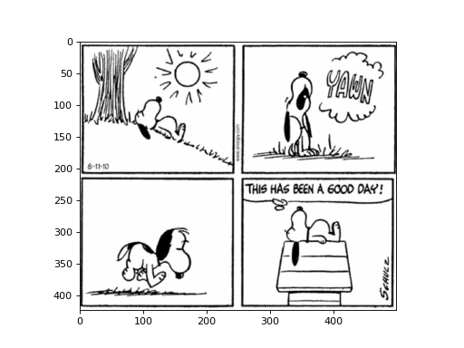
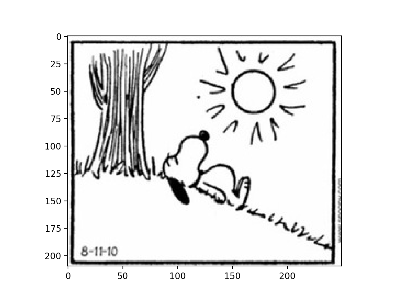
Once we have looked at the image, we have identified that our interest lies solely in a specific portion of the image (perhaps only the first panel of the comic). Let’s create a function that takes the image as input and produces a new image containing only the desired part.
For this task, we need to extract a part of the original image. This can be achieved by performing slicing of the original image.
- Write a function
extract_subimage()that accepts the image as input and returns a new image containing only a part of the original. Your function should take the image, the upper left corner of the sub-image, and a size (rows \(\times\) columns) as input, and it should return a new image containing the pixels from the starting point to the starting point + size. Assume a 2D array as input, and that all pixels in the sub-image are within the image.
For example if we want only the first panel of the comic, we can call the function like this:
img = np.load('cp/ex11/files/comic.npy')
subimage = extract_subimage(img, (0, 0), (210, 250))
plt.imshow(subimage, cmap='gray')
plt.show()
(Source code, png, hires.png, pdf)

Add your function to the file cp/ex11/extract_subimage.py to run the tests.
- cp.ex11.extract_subimage.extract_subimage(image, start_point, size)#
Extract a subimage from an image.
- Parameters
image (
ndarray) – Image to extract from.start_point (
tuple) – Coordinates of the top left corner of the subimage.size (
tuple) – Size of the subimage.
- Return type
ndarray- Returns
Subimage.
Exercise 11.7: Bacteria: Growth#
Exercise 11.7: Bacteria: Growth
Let’s take a look at the experiment data from Exercise 8 again and analyze the data using NumPy. We will start by looking at which time-point the threshold was exceeded (like in Exercise 8.9) and plot the time-points in a histogram. This time, we want to know the time-point of each experiment and not the average time-point of all experiments.
Start by loading the data from the files into a 2D array. Each row in the array should contain the data from one experiment. You can read a file directly to an array using the function np.loadtxt().
Write a function load_data(), that returns a 2D array containing all the experiments.
Tip
Remember that you can loop over the files like this:
for i in range(160):
    filename = f'cp/ex08/files/experiments/experiment_{i:03}.csv'
    data[i] = np.loadtxt(filename, delimiter=',')
This will be the only time today you need to use a for-loop.
Remember to preallocate your numpy array before the loop.
Once you have loaded the data, we want to find the time-point when the threshold was exceeded for each experiment. Write a function threshold_exceeded(), that takes the data as input and returns a 1D array containing the time-point when the threshold was exceeded for each experiment.
Tip
You can use the function np.argmax() to find the index of the first element that is larger than a given value. You can assume that the threshold is always exceeded at some time-point.
Plot a histogram of when a certain threshold was exceeded. You can use the function plt.hist() to plot a histogram. Try if you can get a histogram that looks like this:
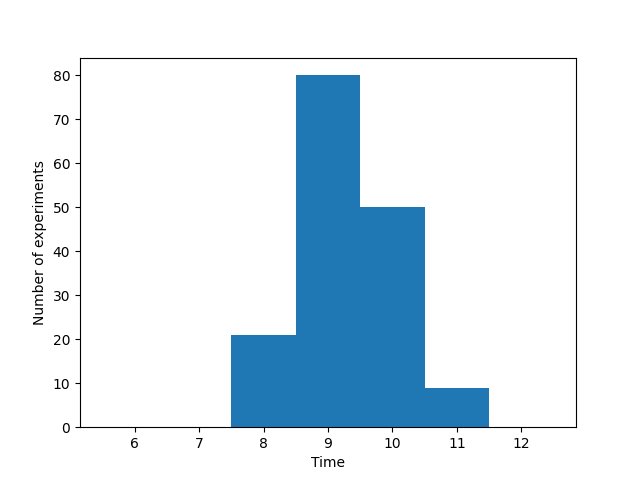
Histogram of when the threshold was reached for each experiment.#
Help for plotting
You can plot a histogram like this:
import matplotlib.pyplot as plt

data = load_data()
threshold_time =  threshold_exceeded(data, 8.5)
plt.hist(threshold_time, bins=[5.5, 6.5, 7.5, 8.5, 9.5, 10.5, 11.5, 12.5])
plt.show()
Add your functions to the file cp/ex11/bacterial_growth.py and run the tests to check if your functions are correct.
- cp.ex11.bacterial_growth.load_data()#
Load data from 160 files into one array. Files are located in cp/ex11/files/experiments.
- Return type
ndarray- Returns
The data from the files in one array.
- cp.ex11.bacterial_growth.threshold_exceeded(data, threshold)#
Return the index at which the threshold is exceeded for each experiment.
- Parameters
data (
ndarray) – The data to search.threshold (
float) – The threshold to compare against.
- Return type
ndarray- Returns
The index at which the threshold is exceeded for each row.
Exercise 11.8: Bacteria - Average growth curve#
Exercise 11.8: Bacteria - Average growth curve
Calculate the mean and standard deviation for each time point (i.e., each column).
Implement the functions get_mean() and get_std() in the file cp/ex11/bacterial_growth.py to run the tests.
Plot the mean and std. Try to make a plot that looks like this:
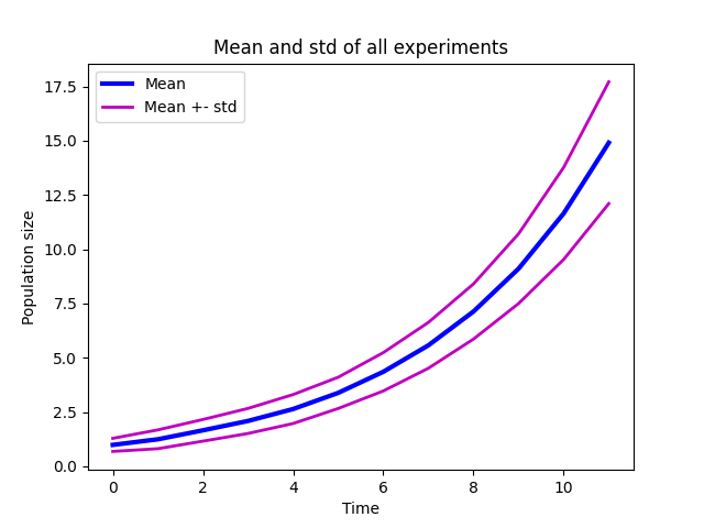
Mean growth curve with standard deviation.#
Help for plotting
You can plot the mean and std like this:
import matplotlib.pyplot as plt

data = load_data()
mean = get_mean(data)
std = get_std(data)
plt.plot(mean)
plt.plot(mean - std, 'm', mean + std, 'm')
plt.legend(['Mean', 'Std'])
plt.show()
- cp.ex11.bacterial_growth.get_mean(data)#
Calculate the mean of the data.
- Parameters
data (
ndarray) – The data to calculate the mean of.- Return type
ndarray- Returns
The mean of the data for each time-point.
- cp.ex11.bacterial_growth.get_std(data)#
Calculate the standard deviation of the data.
- Parameters
data (
ndarray) – The data to calculate the standard deviation of.- Return type
ndarray- Returns
The standard deviation of the data for each time-point.
Exercise 11.9 Bacteria - Outliers#
Continuing with the bacteria data, we will now look for outliers. An outlier is a data point that stands out significantly from the rest of the data.
Here we will identify outliers, by looking at the bacteria count at the last time-step across all experiments.
An experiment is considered an outlier if its final bacteria count, is more than two standard deviations from the mean of all experiments’ final counts. You can use the function get_mean() and get_std() from the previous exercise to calculate the mean and standard deviation.
Therefore, you should write a function that examines data and returns
a numpy array with the experiment index (the number in the filename) of the outlier experiments.
The function should be able to handle data of any size, that is any number of experiments and any number of time-steps.
You can use np.where to convert from a boolean array to an array of indices.
Add your function to the file cp/ex11/outliers.py to be able to test and hand-in your solution.
- cp.ex11.outliers.outliers(data)#
Return the outliers of a dataset.
- Parameters
data (
ndarray) – The data to search.- Return type
ndarray- Returns
The outliers of the data.
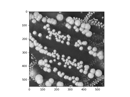
Exercise 11.10 Image Area#
Here is an image of the bacteria, located in cp/ex11/files/bacteria.npy
We want to calculate how much of the image is covered by bacteria. We consider only pixels with a value over 100 to be bacteria.
(Source code, png, hires.png, pdf)

Hint
Apply a threshold of 100 to create a binary image consisting of ones and zeros, determined by pixel intensity. By computing the mean of this binary image, you can calculate the fraction of the image occupied by bacteria (where pixel intensity is greater than 100)
Add your function to the file cp/ex11/bacterial_area.py to be able to test and hand-in your solution.
- cp.ex11.bacterial_area.bacterial_area(npy_path)#
Calculate the fraction of the image where pixel intensities are greater than 100.
Parameters: :type npy_path:
str:param npy_path: Path to the image data file in NumPy format. :rtype:float:return: The fraction of area in an image where there are bacteria.